Most information systems log events (e.g., in transaction logs, audit trails) to audit and monitor the processes they support. Proper analysis of these process execution logs can yield important knowledge and help organizations improve the quality of their services. The Decision Miner analyzes how data attributes influence the choices made in the process based on past process executions. More precisely, it aims at the detection of data dependencies that affect the routing of a case. The approach is based on machine learning techniques, and the Decision Miner uses algorithms implemented in the Weka [1] library to solve the classification problem.
This plug-in expects a process model (as a Petri net) and its process execution log already being tied together, which can be achieved in two different ways.
The first possibility is to
- open the log file (in MXML format), and
- open a process model, whereas the log must be connected to the log during the import of the process model via choosing File → Open [process format] file → With: [log] from the menu.
The process model must either be available in some Petri net format (a .tpn or .pnml file) or in another modeling paradigm that can be read by ProM (such as an EPC or a YAWL model), which can then be converted into a Petri net by dedicated conversion plug-ins within the framework.
The second possibility can also be applied if no process model is available beforehand, but instead the model is first to be discovered using some process mining algorithm. This approach is demonstrated in the following. You can follow the procedure if you open the example log for the decision miner, which is located in the examples/decisionMining/ folder of your ProM directory (or can be downloaded here ).
- Open the file DecisionMinerExampleLog.xml via choosing File → Open MXML Log file from the menu.
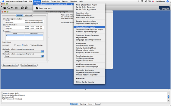
- Choose a process mining algorithm, for example: Mining → Filtered exampleLog.xml → Alpha algorithm plugin (see Figure 1).
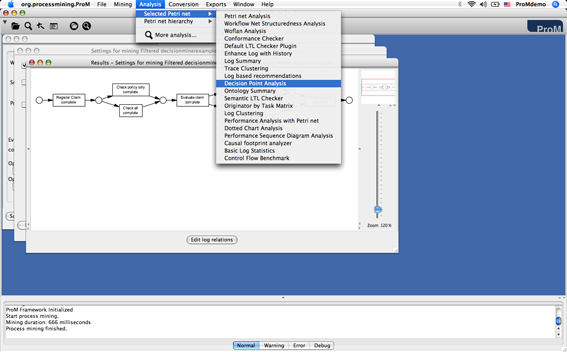
- The process model for the example log has been discovered, and attached to the log. Now you can invoke the Decision Miner choosing Analysis → Selected Petri net → Decision Point Analysis from the menu (see Figure 2).
When the Decision Miner starts up, it determines all the decision points in the process model and displays them in the upper left corner of the application window. The idea is to convert every decision point into a classification problem [1,2], whereas the classes are the different decisions that can be made. As training examples we can use the process instances in the log (for which it is already known which alternative path they have followed with respect to the decision point). The attributes to be analyzed are the case attributes contained in the log.
On the upper right side several views can be selected, which are briefly described in the following before starting the actual analysis.
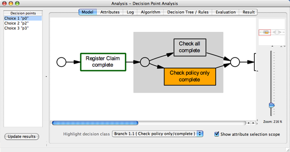
Model ViewThe model view visualizes a choice construct (that is, in Petri net terms a place with more than one outgoing arcs) within the process model. In Figure 3, decision point p0 is depicted in a gray box. In the example process, which represents a simple insurance claim handling process, this choice reflects the decision about whether a full check needs to be performed after the initial registration step, or whether a policy-only check is sufficient for that case. Furthermore, one of the alternative branches has been selected (in the combo box Highlight decision class), which fills the first task in that branch (here “Check policy only”) with orange color. Finally, the Show attribute selection scope option has been chosen, which marks all those tasks with green line color whose attributes are to be considered for the data dependency analysis for this decision point. In the example process only the previous task “Register Claim” is highlighted, and therefore only attributes provided by this task are taken into account for the decision point analysis.
The log view provides a means to manually inspect the process instances categorized with respect to the decisions made at each decision point in the model. In Figure 4, the decision point p0 of the example process is assessed according to the alternative branches “Check all” (which has been followed by two out of six cases) and “Check policy only” (which has been followed by four out of six cases), and process instance Case 2 is currently being displayed in the right-most window. One can observe that during the execution of activity “Register Claim” information about the amount of money involved (Amount), the corresponding customer (CustomerID), and the type of policy (PolicyType) are provided. Semantically, Amount is a numerical attribute, the CustomerID is an attribute which is unique for each customer, and both PolicyType is an enumeration type (being either “normal” or “premium”).

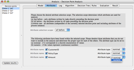
The attributes view allows for the selection of those attributes to be included in the analysis of each decision point. In Figure 5, this view shows all the attributes that are available in the current selection scope for the choice p0. Per default this includes all activities that have been executed before the decision point is reached (with respect to p0 this only includes the task “Register Claim”). However, the scope can be changed in order to include all attributes of the whole case if needed. For the example process, keep the default selection scope and all the attributes included. Furthermore, the type of each attribute can be determined to enable a correct interpretation. Currently, the types nominal and numeric can be distinguished. For the example process, set the type of the Amount attribute to be numeric.
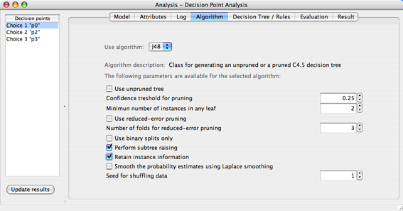
While the Decision Miner formulates the learning problem, it is solved with the help of data mining algorithms provided by the Weka software library [1]. The algorithm view allows for the selection of the data mining algorithm to be used for the analysis of a decision point. Currently, only the decision tree algorithm J48, which is the Weka implementation of an algorithm known as C4.5 [2] is supported. The parameters are further explained by help texts when hovering above the respective option. In order to follow the running example, keep the default parameters, but enable the option Retain instance information (this will provide some additional visualization options as soon as the result has been calculated), as shown in Figure 6.
Now we are ready to invoke the analysis. By pressing the button Update results a decision tree is being created for each decision point by the classification algorithm J48. The following section shows how it can be interpreted in order to derive knowledge about what attributes have most likely influenced the corresponding choices.
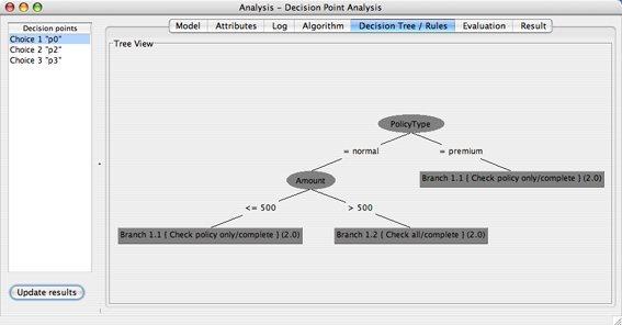
Decision Tree ViewThe Decision Tree view visualizes the result obtained for each decision point, and depending on the algorithm chosen for the analysis.
Figure 7 shows the decision tree result of the J48 algorithm with respect to the choice p0. From the depicted tree one can now infer the logical expressions that form the decision rules for the decision point p0 in the following way. If an instance is located in one of the leaf nodes of a decision tree, it fulfills all the predicates on the way from the root to the leaf, i.e., they are connected by a boolean AND operator. For the example process, the branch “Check all” is chosen if (PolicyType = “normal”) AND (Amount > 500). When a decision class is represented by multiple leaf nodes in the decision tree the leaf expressions are combined via a boolean OR operator. Therefore, the branch “Check policy only” is chosen if ( (PolicyType = “normal”) AND (Amount ≤ 500) ) OR (PolicyType = “premium”), which can be reduced to (PolicyType = “premium”) OR (Amount ≤ 500). This means that the extensive check (activity Check all) is only performed if the amount is greater than 500 and the policy type is “normal”, whereas a simpler coverage check (activity “Check policy only”) is sufficient if the amount is smaller than or equal to 500, or the policyType is “premium”, which may be due to certain guarantees by “premium” member corporations.
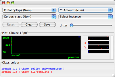
If you have chosen the option to retain the instance information before starting the analysis (see Figure 6), you may use additional visualization options to explore the result for a decision point analysis by right-clicking any node in the decision tree.
Furthermore, you can export the classification problem for the corresponding decision point as an .arff file (just click on the top-node in the decision tree and press “Save” in the dialog shown in Figure 8), which can then be loaded into the Weka workbench to see which results are given by other classifiers not yet supported by the Decision Miner. Try, for example, a rule learner such as JRip, which will discover If-then rules rather than a decision tree.
The Evaluation view tells you how many decisions were correctly (or incorrectly) captured by the discovered rule. Therefore, it provides an indication of the “accuracy” of the discovered rules. Figure 9 shows the evaluation results for the decision tree shown in Figure 7: for the decision point p0 all the cases in the log could be correclty classified by the decision tree classifier. For further information about the other statistics, please refer to the Weka documentation [1].

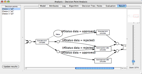
The Result view visualizes the discovered rules (and the selected data attributes) in the context of the process model. Note that the rules discoverd by the Decision Miner can be included in a simulation model of your process. See this page for further information on simulation models in ProM.
Note that the Decision Miner is able to deal with process models containing both invisible and duplicate activities. However, if an alternative branch contains only invisible or duplicate activities, it cannot be detected as a decision class either.
For further details please refer to [3].
Since ProM 5.0 there is a simple way to deal with loops: A new button called “Loop-split Log” allows to export a new log file that splits up process instances that contain several decisions with respect to the current decision point (due to the presence of loops) within one case into multiple process instances. Because the Decision Miner always interprets the last value of an attribute within the scope, these different instances can now serve as multiple learning instances. Export and re-import the loop-split log, connect it to the analyzed process model, and then re-analyze that particular decision point.
References[1] I. H. Witten and E. Frank. Data Mining: Practical machine learning tools and techniques, 2nd Edition . Morgan Kaufmann, 2005.
[2] J. R. Quinlan. C4.5: Programs for Machine Learning. Morgan Kaufmann, 1993.
[3] A.Rozinat, W.M.P. van der Aalst. Decision Mining in Business Processes. BPM Center Report BPM-06-10, BPMcenter.org, 2006.
[4] A.Rozinat, W.M.P. van der Aalst. Decision Mining in ProM. In S. Dustdar, J.L. Fiadeiro, and A. Sheth, editors, BPM 2006, volume 4102 of Lecture Notes in Computer Science, pages 420–425. Springer-Verlag, Berlin, 2006.