Allows to view and manually manipulate high-level information, which can be directly used in the creation of simulation models.
This view remains the same for all high-level processes. That is, regardless the underlying control-flow model extra information about data, time and resources can be provided (only the visualization at the bottom will change).
This plug-in becomes available in the Analysis menu as soon as one of the following objects is provided:
- A high-level process, such as a HLYAWL, HLPetrinNet, or HLActivitySet object.
- A plain YAWL model (a HLYAWL model will be created).
- A plain PetriNet model (a HLPetriNet model will be created).
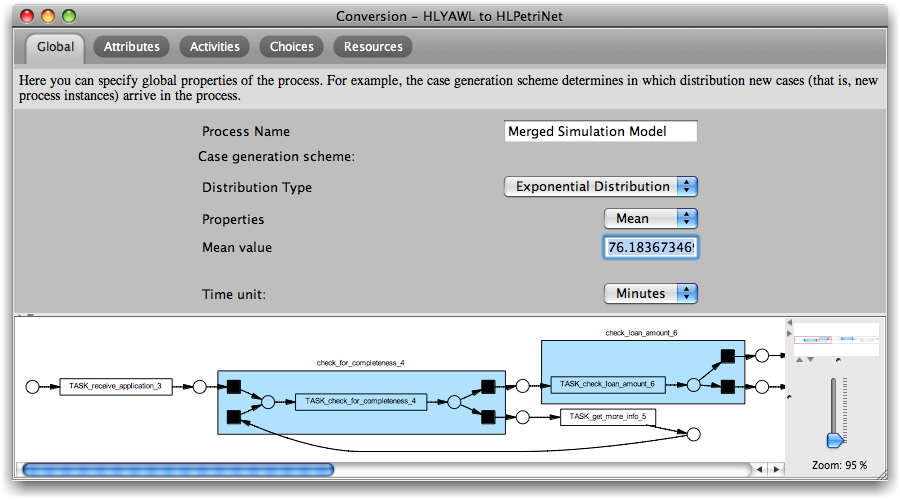
On the “Global” tab process-wide settings can be adjusted. The following parameters are available:
- Case generation scheme: Specifies the distribution at which new cases arrive in this process. Typically this is a negative exponential distribution that can be specified via the mean (time between two arrivals).
- Time unit: Global time unit that applies to all time-related parameters. This affects the MXML logging during simulation.
The “Attributes” tab allows to modify or delete existing and create further data attributes. Each attribute can have the following parameters:
- Name: The name of the data attribute. Should be globally unique to avoid confusion.
- Type: Attributes can be of either the type “nominal”, “numeric”, or “boolean”.
-
Use initial value: Determines whether there should be an
initial value used in the first place.
- If yes, the actual initial value can be specified.
- If not, the attribute will be initialized with a random value from the possible values during simulation. This is useful for global case data attributes, which are used for decision making (see also Choice Settings) but never modified by any activity.
- Initial value: Specifies the actual initial value, if used.
- Possible values: Defines the range of possible values, depending on the attribute type.

Note that double-clicking an attribute in the list will bring up the current parameters as well as highlight all those activities in the visualization below that provide this attribute (see also Activity Settings).
Choice SettingsDecision points in the process model are automatically detected and displayed in the list to the left (and highlighted in the process model at the bottom). For each of these choices, the following options exist.
- unguided (random): The choice can be made completely random. CPN Tools will randomly choose between enabled branches.
- data attributes: Based on logical expressions over data attributes pre-conditions can be formulated (see also Attribute Settings). Currently, these rules can be discovered by the (Decision Miner ) or imported (newYAWL Import) but not yet manually provided. So, the fields cannot be edited.
- probabilities: A probability can be assigned to each of the alternative branches. Make sure they add up to 1.
- frequencies: If choices are not independent of each other then simple probabilities cannot be specified (see this publication for further details). In these situations, relative frequencies can determine how often each of the branches is chosen with respect to the others instead.

The “Resources” tab allows to provide information about organizational entities (groups) and individual resources belonging to one or more of these groups. Organizational models can be directly imported (see OrgModel Import) or manually specified here.
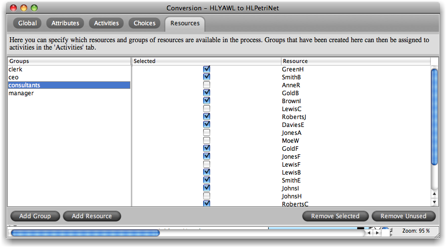
Note that these groups can be used to define required roles for activities (see also Activity Settings), and that unused roles (i.e., groups that are assigned to no activity in the process) can be removed by pressing the button “Remove Unused”.
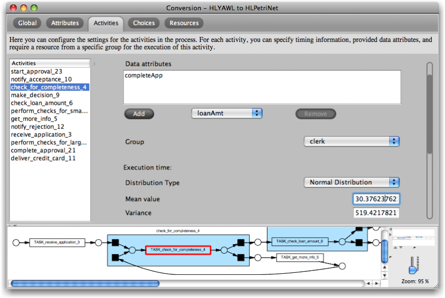
Activity SettingsThe “Activities” tab holds information for each activity in the process. Double-clicking an activity in the list brings up the activity settings, plus it highlights the corresponding node in the graphical model at the bottom. For each activity the following parameters can be specified:
- Data attributes: Output data items (see also Attribute Settings) can be added or removed. When an attribute in this view is selected, it can be chosen to be either “resampled” (new value is generated based on value range distribution) or “re-used” (value is not changed but attribute will be logged with execution of this activity).
- Group: A group can be chosen from the list of organizational entities (see also Resource Settings). Furthermore, an activity can be chosen to be executable by “nobody” (automatic task - no resource is required) or “anybody” (any available resource will do).
- Execution time: A distribution can be specified for the actual execution of this activity (i.e., from start to completion).
- Waiting time: A distribution of the time after becoming enabled but before actually starting the activity can be specified (i.e., from scheduling to start).
- Sojourn time: The sojourn time is the execution time + waiting time for an activity (i.e., from scheduling to completion). This can be useful if the timing behavior is discovered from a log that did not contain information about the actual start of activities (like common, e.g., for Staffware logs).